Causal discovery examples
I) Data analysis (fixed data)
The following example falls into scenario I) Data analysis (fixed data) of the Data scenarios.
Sachs et al. 2005 data
Config file: config/realistic_study.json.
Command:
snakemake --cores all --use-singularity --configfile config/realistic_study.json
We show estimation results for the logged and standardized version (2005_sachs_2_cd3cd28icam2_log_std.csv) of the second dataset anti-CD3/CD28 + ICAM-2 from Sachs et al.[1] with 902 observations. The data is visualised in Fig. 1 with pairwise scatter plots using the ggally_ggpairs module.
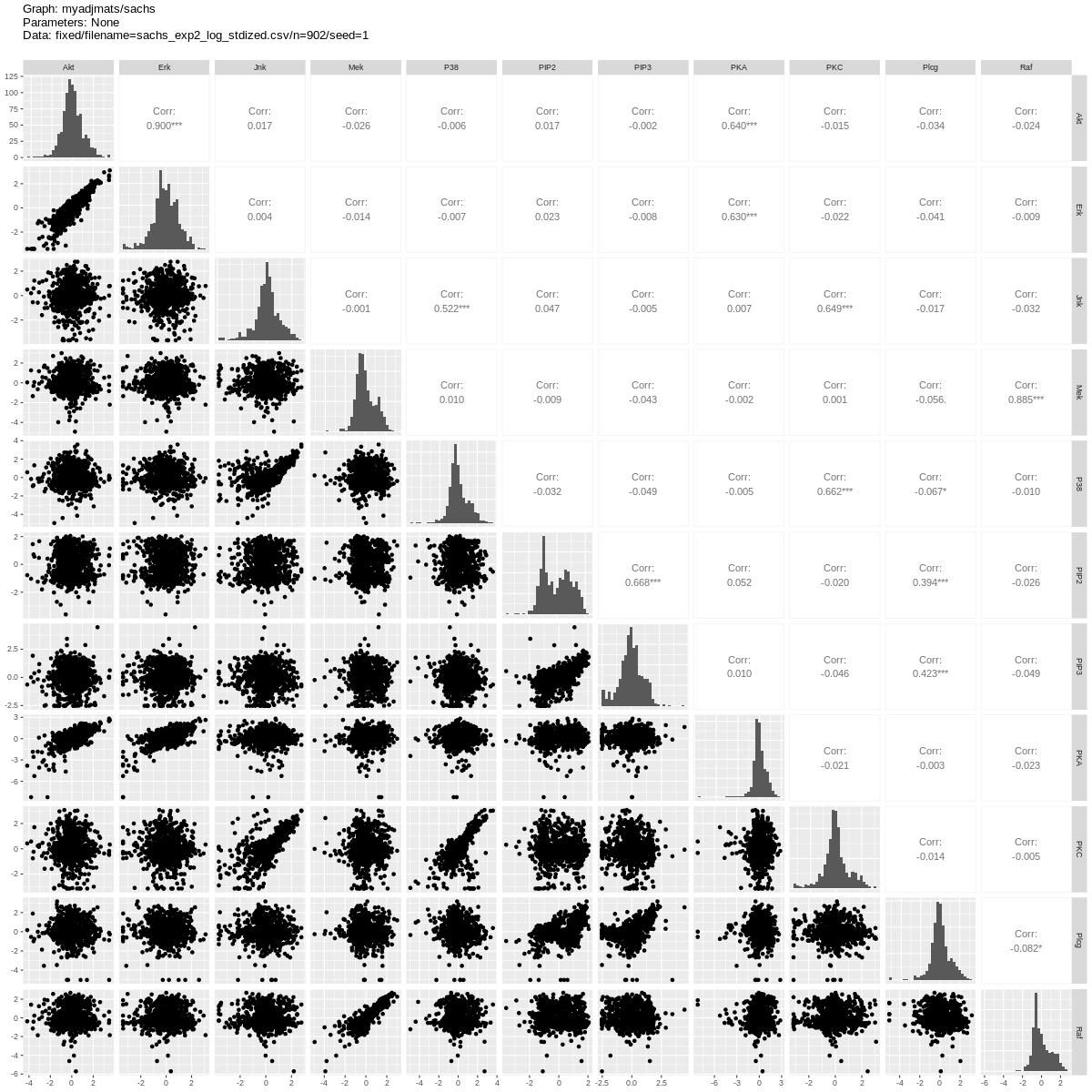
Fig. 1 Scatter plots for the logged and standardized Sachs et al. 2005 second dataset (anti-CD3/CD28 + ICAM-2).
Listing 1 shows the benchmark_setup section of the config file.
 1"benchmark_setup": [{
 2    "title": "real_data",
 3    "data": [
 4        {
 5            "graph_id": null,
 6            "parameters_id": null,
 7            "data_id": "2005_sachs_2_cd3cd28icam2_log_std.csv",
 8            "seed_range": null
 9        }
10    ],
11    "evaluation": {
12        "ggally_ggpairs": true,
13        "graph_estimation": {
14            "ids": [
15                "fges-sem-bic",
16                "tabu-bge",
17                "itsearch-bge",
18                "pc-gaussCItest"
19            ],
20            "convert_to": ["cpdag"],
21            "graphs": true,
22            "adjmats": true,
23            "diffplots": false,
24            "csvs": true,
25            "graphvizcompare": false
26        },
27        "mcmc_traj_plots": [],
28        "mcmc_heatmaps": [],
29        "mcmc_autocorr_plots": []
30    }
31}]
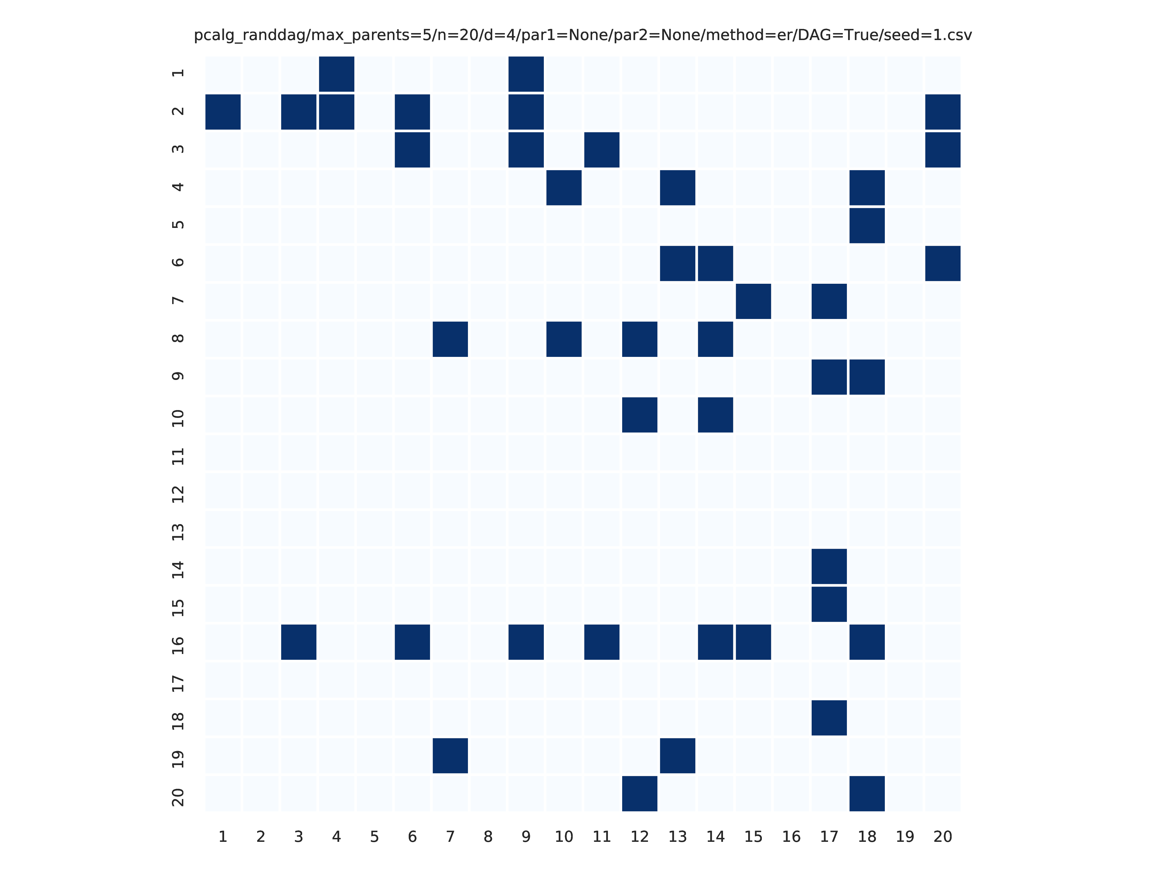
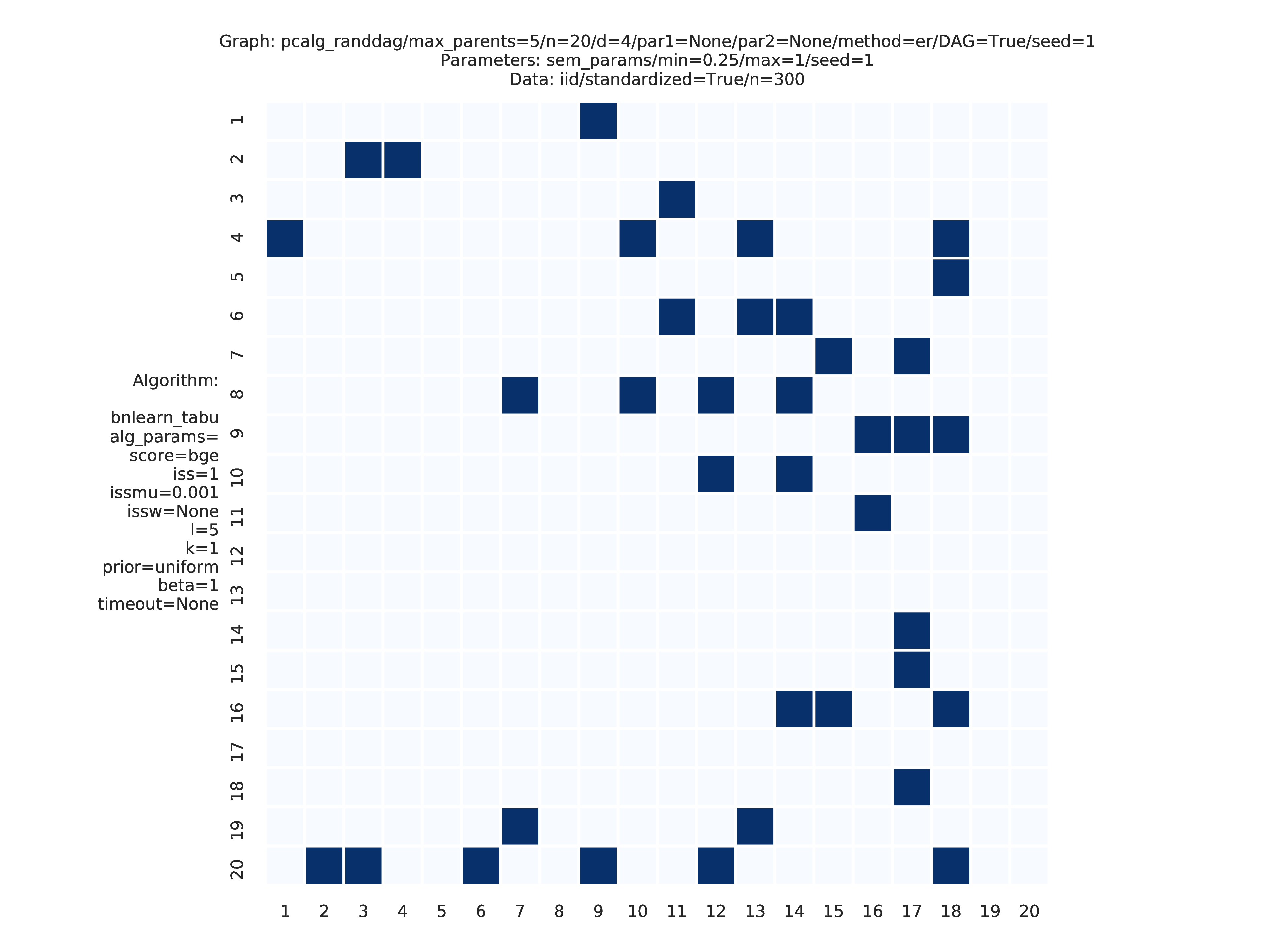
Fig. 2 shows the adjacency matrix produced by the graph_estimation module of the DAG estimated by the Tabu (bnlearn) module.
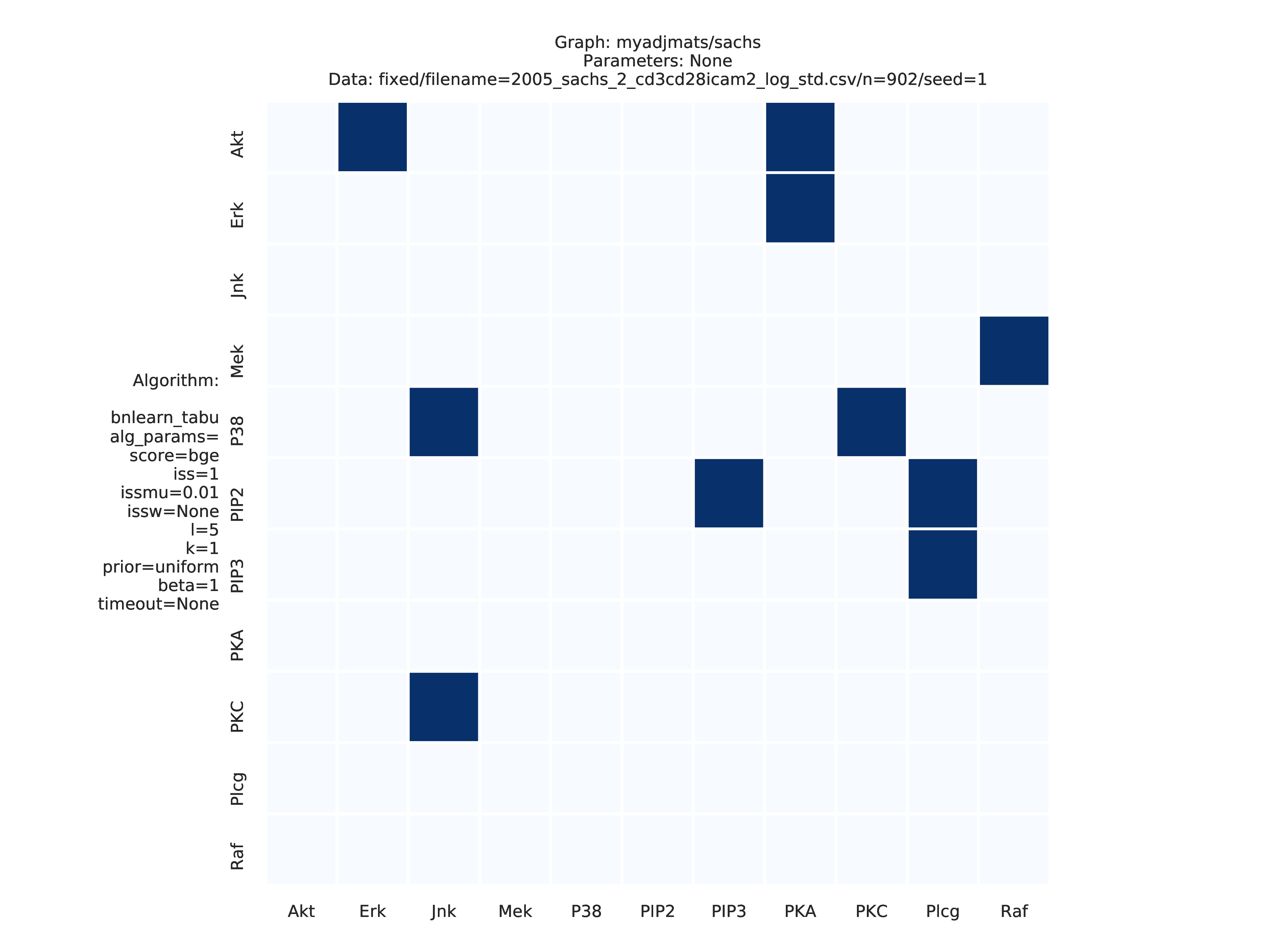
Fig. 2 Estimated adjmat.
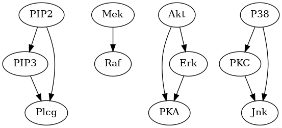
Fig. 3 Estimated graph.
References
II) Data analysis with validation
The following example falls into scenario II) Data analysis with validation of the Data scenarios.
Sachs et al. 2005 data (known graph)
Config file: config/paper_sachs.json.
Command:
snakemake --cores all --use-singularity --configfile config/paper_sachs.json
We show estimation results for the logged and standardized version (2005_sachs_2_cd3cd28icam2_log_std.csv) of the second dataset anti-CD3/CD28 + ICAM-2 from Sachs et al.[1] with 902 observations. The data is visualised in Fig. 1 with pairwise scatter plots using the ggally_ggpairs module.
Listing 2 shows the benchmark_setup section of the config file.
 1"benchmark_setup": [{
 2    "title": "paper_sachs",
 3    "data": [
 4        {
 5            "graph_id": "sachs.csv",
 6            "parameters_id": null,
 7            "data_id": "2005_sachs_2_cd3cd28icam2_log_std.csv",
 8            "seed_range": null
 9        }
10    ],
11    "evaluation": {
12        "benchmarks": {
13            "filename_prefix": "paper_sachs/",
14            "show_seed": false,
15            "errorbar": false,
16            "errorbarh": false,
17            "scatter": true,
18            "path": true,
19            "text": false,
20            "ids": [
21                "gobnilp-bge",
22                "boss-sem-bic",
23                "grasp-sem-bic",
24                "notears-l2",
25                "fges-sem-bic",
26                "hc-bge",
27                "itsearch-bge",
28                "mmhc-bge-zf",
29                "omcmc-bge",
30                "pc-gaussCItest",
31                "tabu-bge"
32            ]
33        },
34        "graph_true_stats": true,
35        "graph_true_plots": true,
36        "ggally_ggpairs": true,
37        "graph_plots": [
38                "gobnilp-bge",
39                "boss-sem-bic",
40                "grasp-sem-bic",
41                "notears-l2",
42                "fges-sem-bic",
43                "hc-bge",
44                "itsearch-bge",
45                "mmhc-bge-zf",
46                "omcmc-bge",
47                "pc-gaussCItest",
48                "tabu-bge"
49        ],
50        "mcmc_traj_plots": [],
51        "mcmc_heatmaps": [],
52        "mcmc_autocorr_plots": []
53    }
54}]
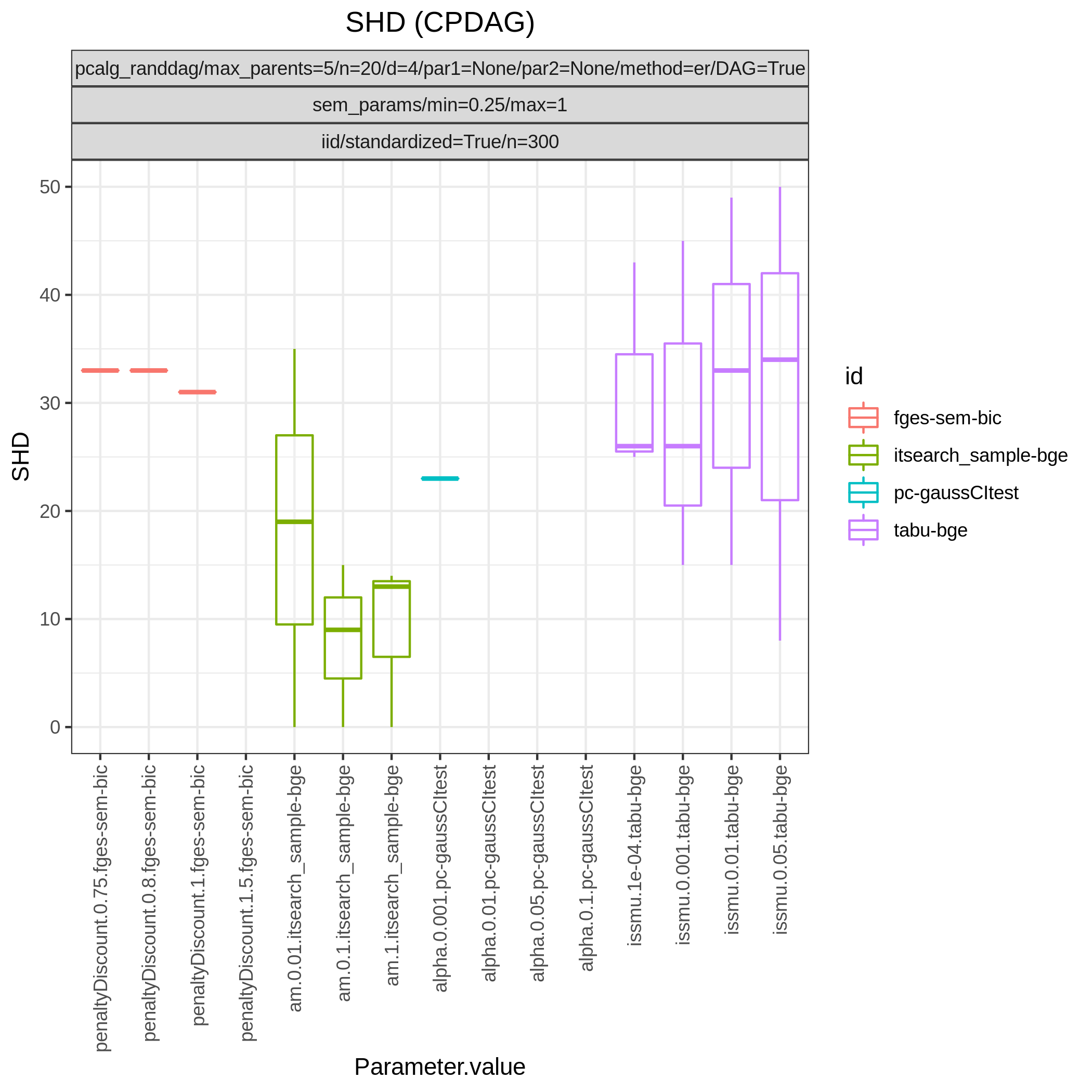
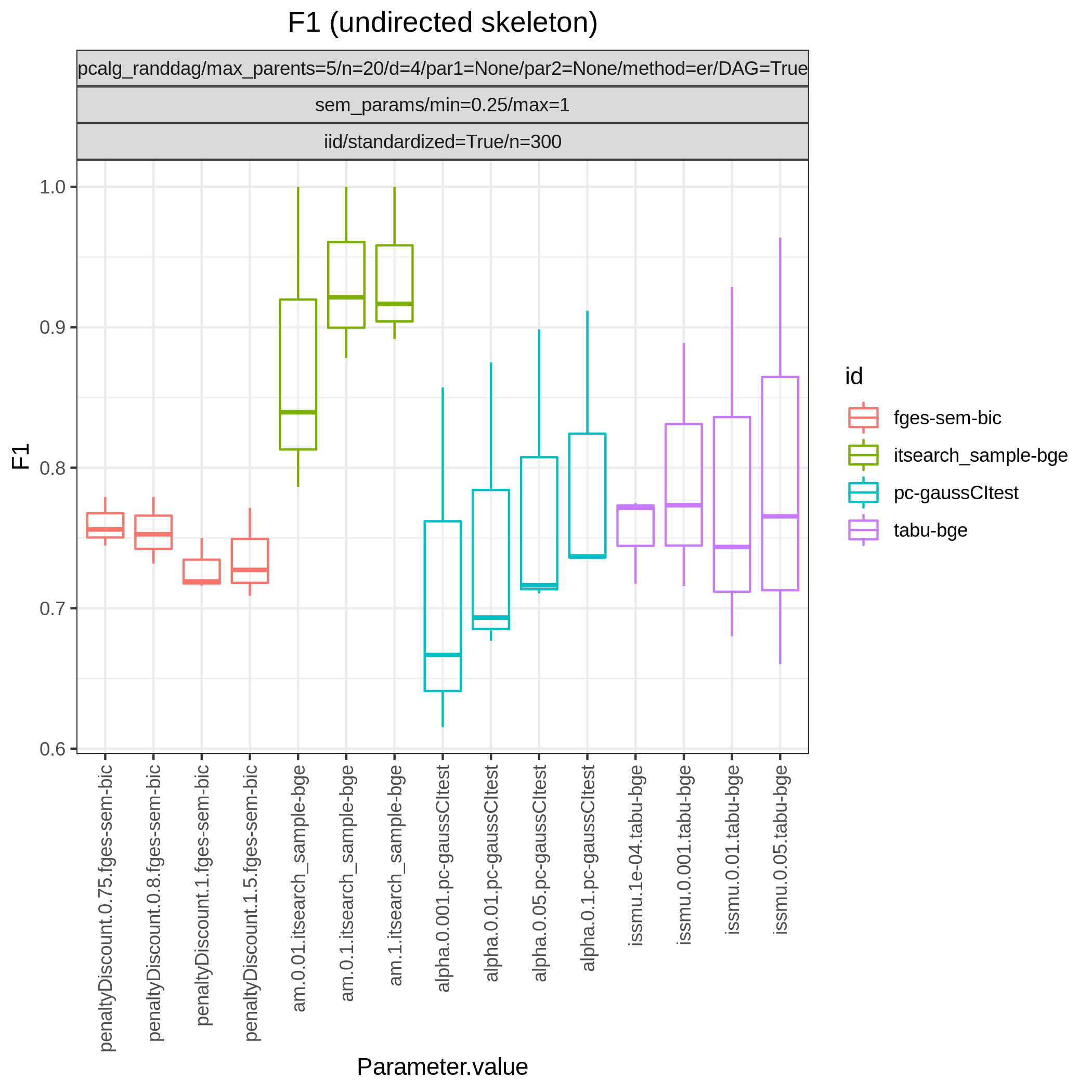
Fig. 4 shows Hamming distance between the edge sets of the true and the estimated CPDAGs (SHD) and the F1 score based on the undirected skeleton from 10 algorithms with different parametrisations, produced by the benchmarks module. From this figure we can directly conclude that all algorithms have a parametrisation that gives the minimal SHD of 9 and maximal F1 score of 0.67.
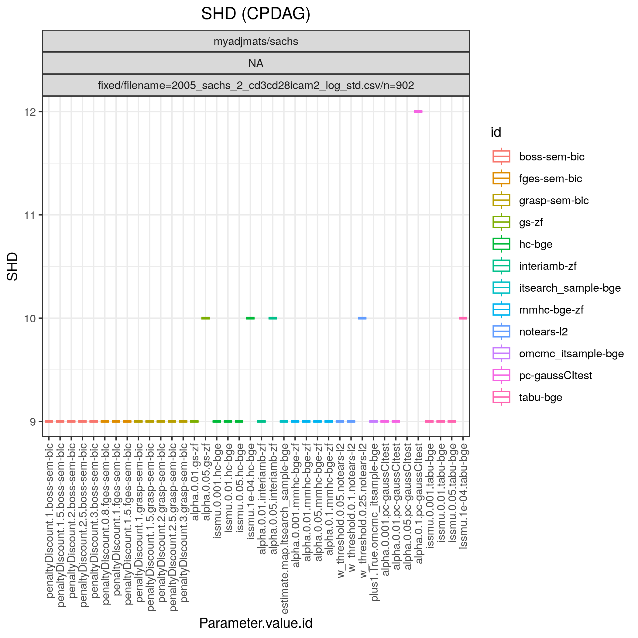
Fig. 4 SHD.
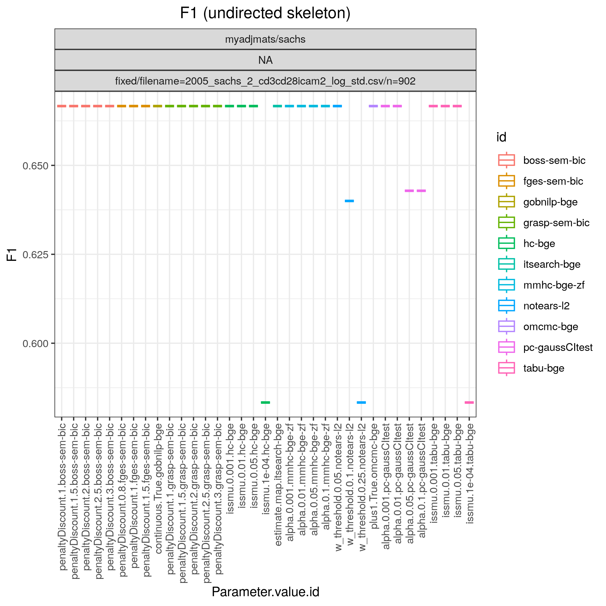
Fig. 5 F1.
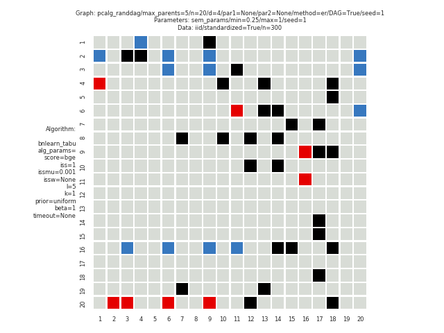
Fig. 6 shows the adjacency matrix produced by the graph_plots module of the DAG estimated by the Tabu (bnlearn) module.
Fig. 6 Estimated adjmat.
Fig. 7 Estimated graph.
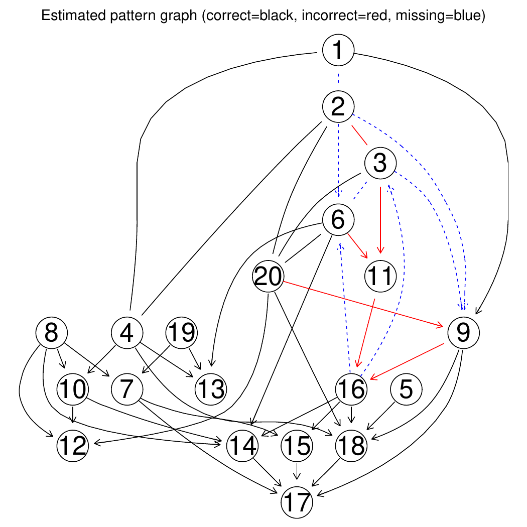
Fig. 8 and Fig. 9 shows the pattern graph of both the true and a DAG estimated by the Tabu (bnlearn) module, where the black edges are correct in both subfigures. The missing and incorrect edges are colored in blue and red respectively in Fig. 9.
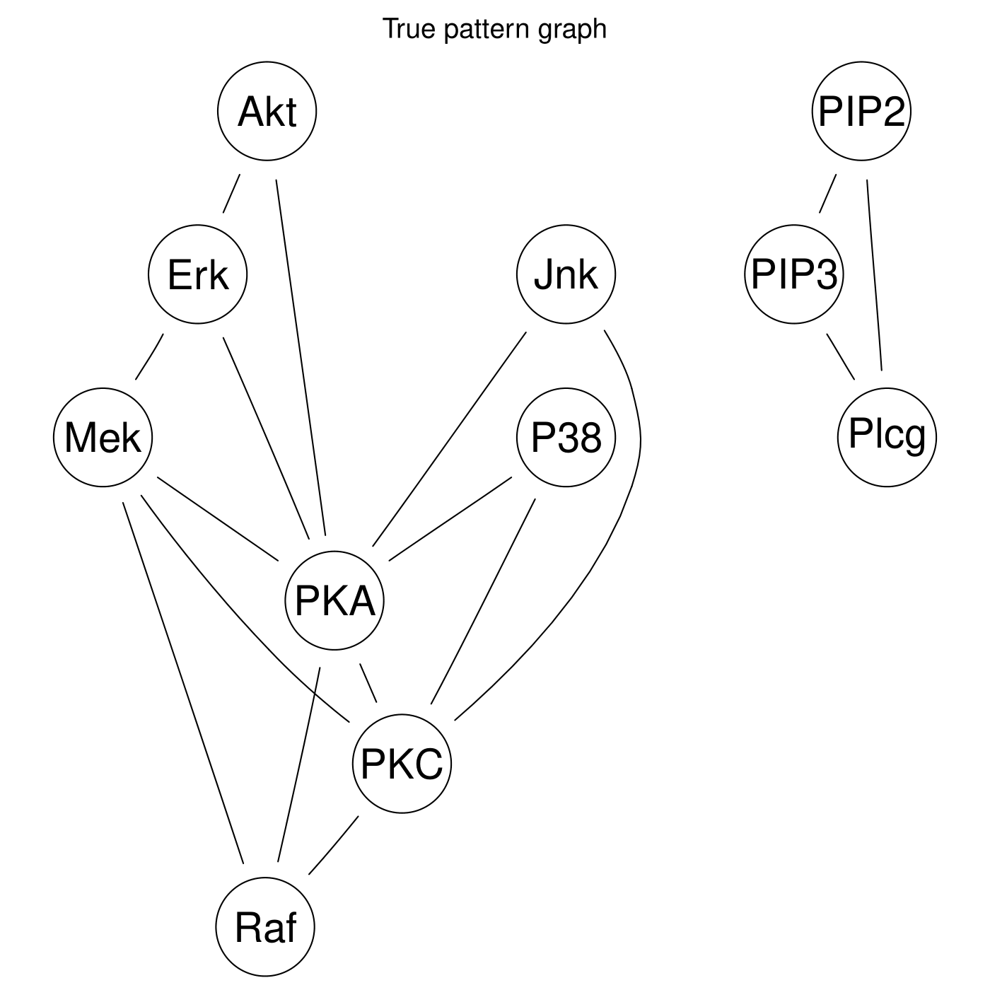
Fig. 8 True pattern graph.
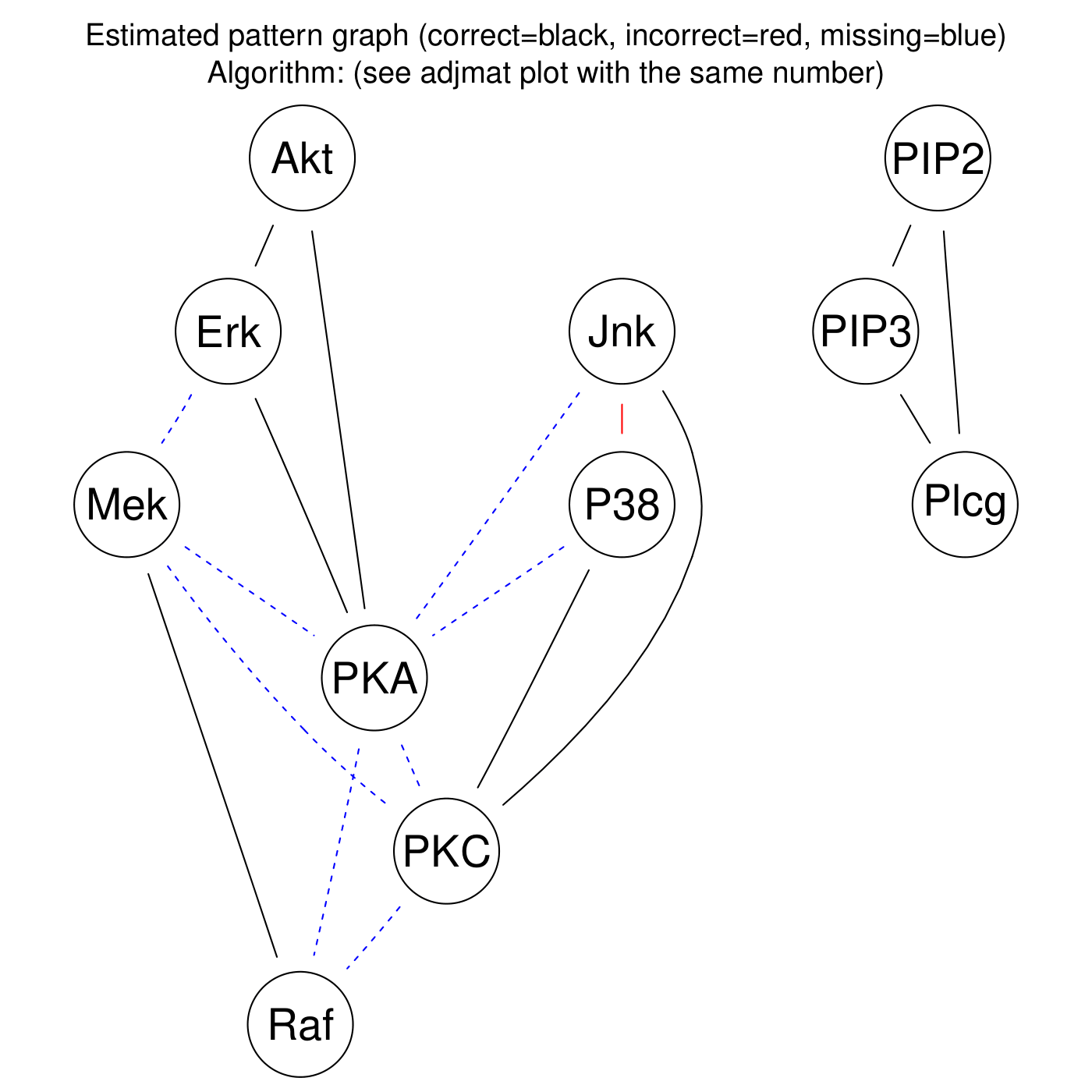
Fig. 9 Diff pattern graph.
References
IV) Fixed graph
The following examples falls into scenario IV) Fixed graph of the Data scenarios.
Random binary HEPAR II network
Config file: config/paper_hepar2_bin.json.
Command:
snakemake --cores all --use-singularity --configfile config/paper_hepar2_bin.json
In this example we study a random binary Bayesian network where the graph \(G\) is fixed and the associated parameters \(\Theta\) are regarded as random. More specifically, we consider 100 models \(\{(G_i,\Theta_i)\}_{i=1}^{100}\), where the graph structure \(G\) is that of the well known Bayesian network HEPAR II (hepar2.csv). This graph has 70 nodes and 123 edges and has become one of the standard benchmarks for evaluating the performance of structure learning algorithms. The maximum number of parents per node is 6 and we sample the parameters \(\Theta_i\) using the bin_bn module, in the same manner as described Random binary Bayesian network. From each model \((G_i,\Theta_i)\) we draw a dataset \(\mathbf Y_i\) of size n=320, using the iid module.
Fig. 10 shows the ROC curves for this scenario. The best performing algorithm is clearly GRaSP (TETRAD) (grasp-sem-bic), followed by BOSS (TETRAD) (boss-sem-bic), FGES (TETRAD) (fges-bdeu), Order MCMC (BiDAG) (omcmc_itsample-bde), Iterative MCMC (BiDAG) (itsearch_sample-bde), all with FP/P \(\approx 0.15.\) The constraint based algorithm PC (pcalg) (pc-binCItest) and MMHC (bnlearn) (mmhc-bde-mi) appear to cluster in the lower scoring region (TP/P <0.4).
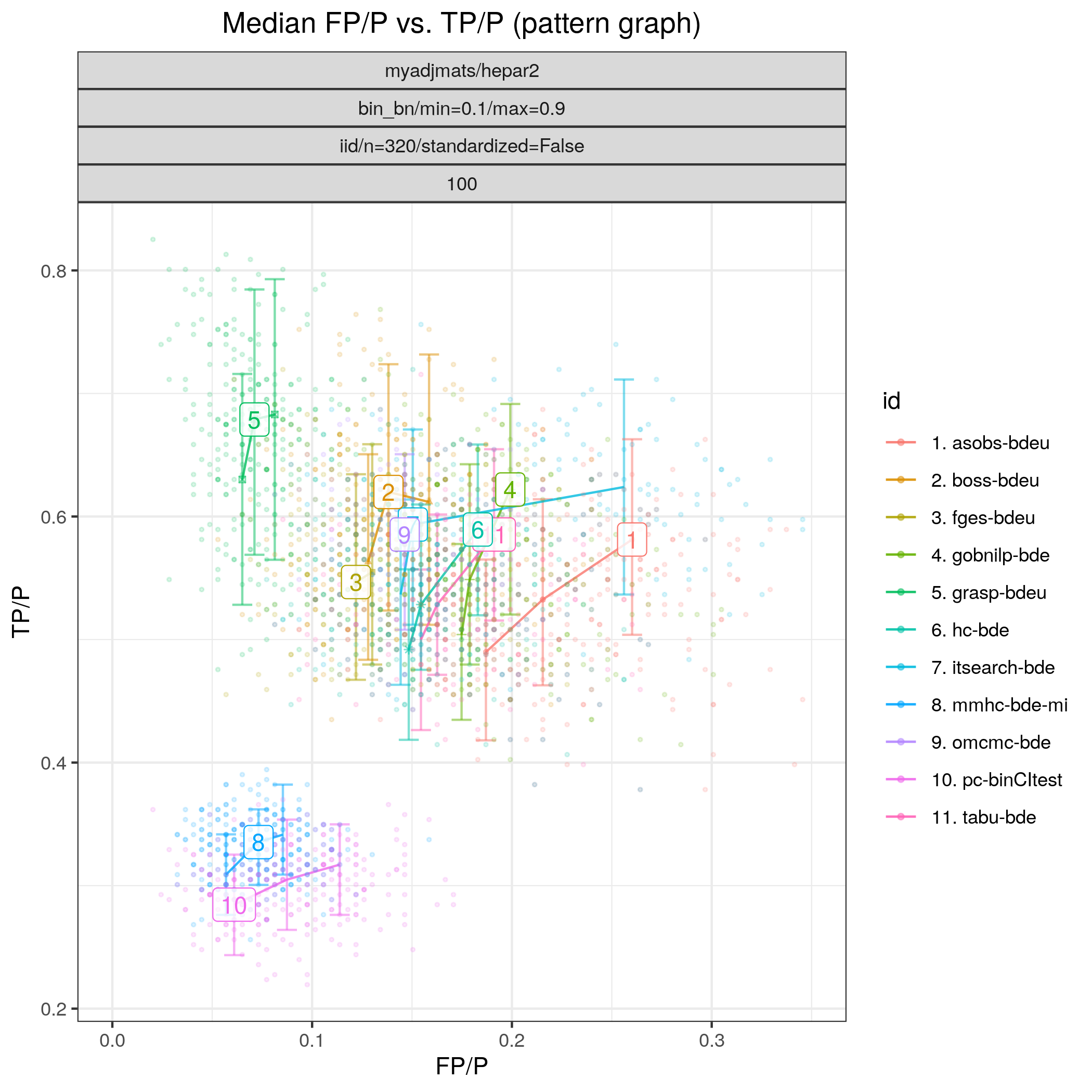
Fig. 10 FP/P vs. TP/P.
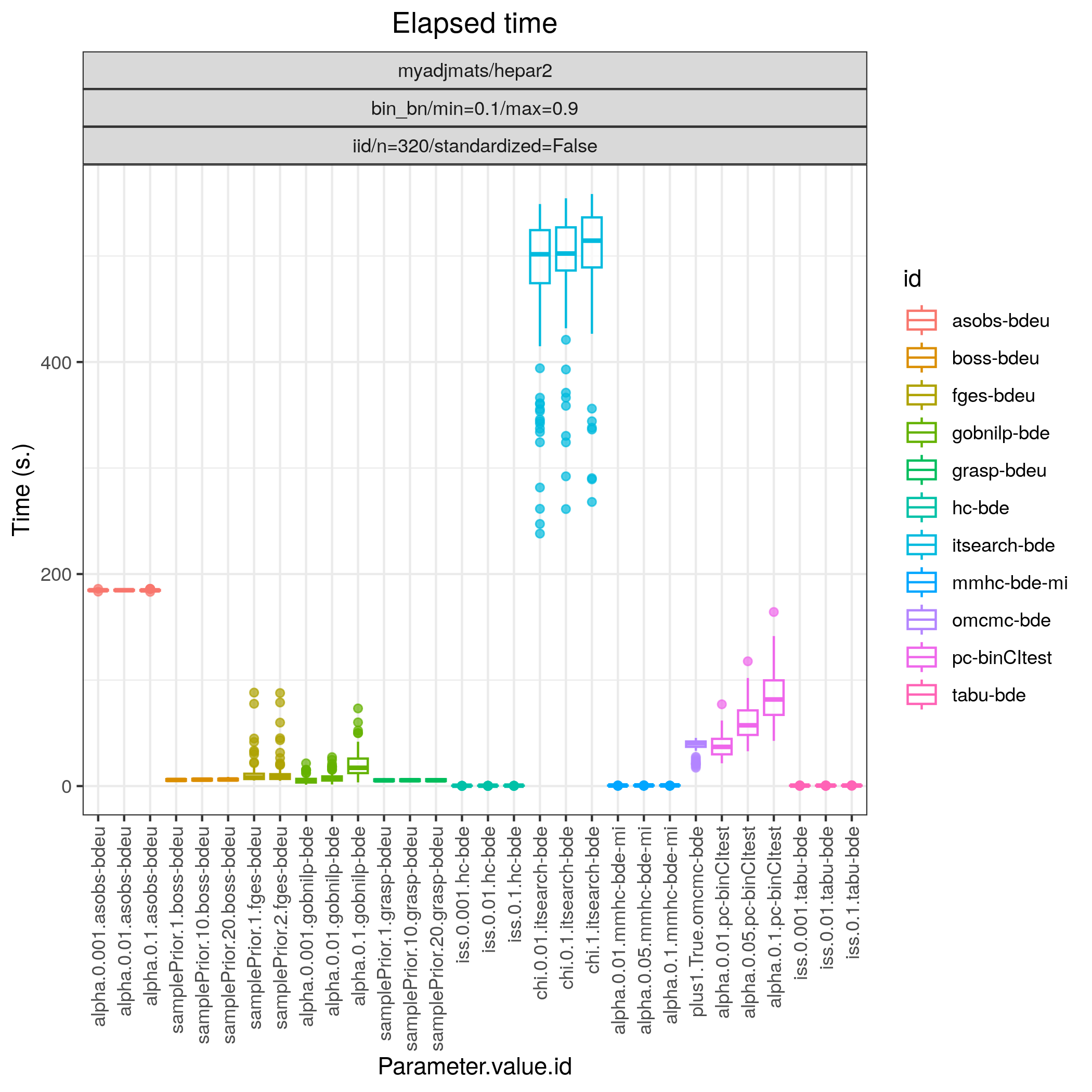
Fig. 11 Timing.
Random Gaussian HEPAR II network
Config file: config/paper_hepar2_sem.json.
Command:
snakemake --cores all --use-singularity --configfile config/paper_hepar2_sem.json
In this example we draw again 100 models \(\{(G_i,\Theta_i)\}_{i=1}^{100}\), where \(G\) corresponds to the HEPAR II network (hepar2.csv), and \(\Theta_i\) are the parameters of a linear Gaussian SEM sampled using the sem_params, module with the same settings as in Random binary Bayesian network. From each model \((G,\Theta_i)\), we draw a standardised data set \(\mathbf Y_i\) of size n=320, using the iid module.
The results of Fig. 12 highlight that GRaSP (TETRAD) (grasp-bdeu) has nearly perfect performande.:abbr: Also BOSS (TETRAD) (boss-bdeu), Order MCMC (BiDAG) (omcmc_itsample-bdeu), Iterative MCMC (BiDAG) (itsearch_sample-bge) separate themselves from the rest in terms of SHD (combining both low FP/P and high TP/P) for both sample sizes.
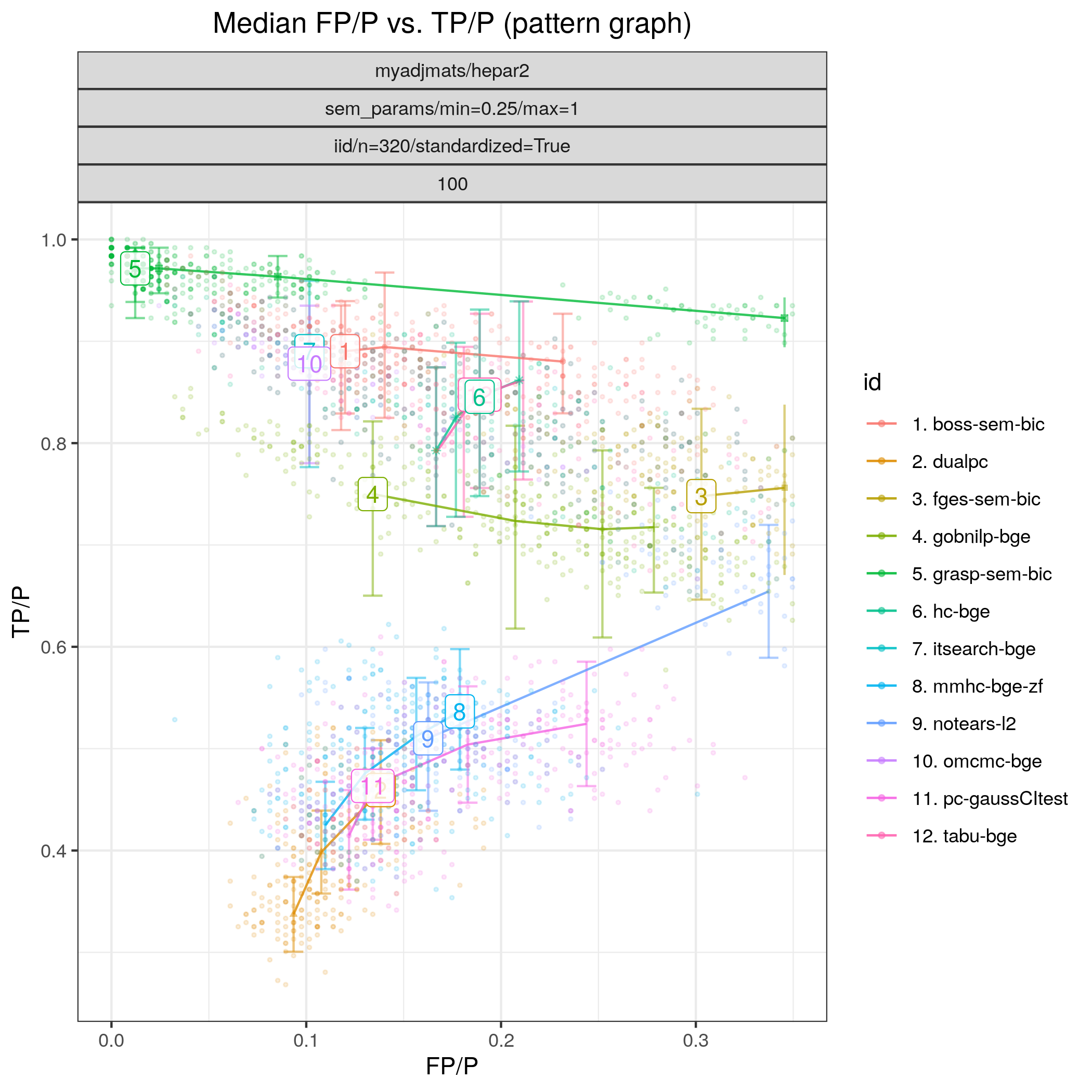
Fig. 12 FP/P vs. TP/P.
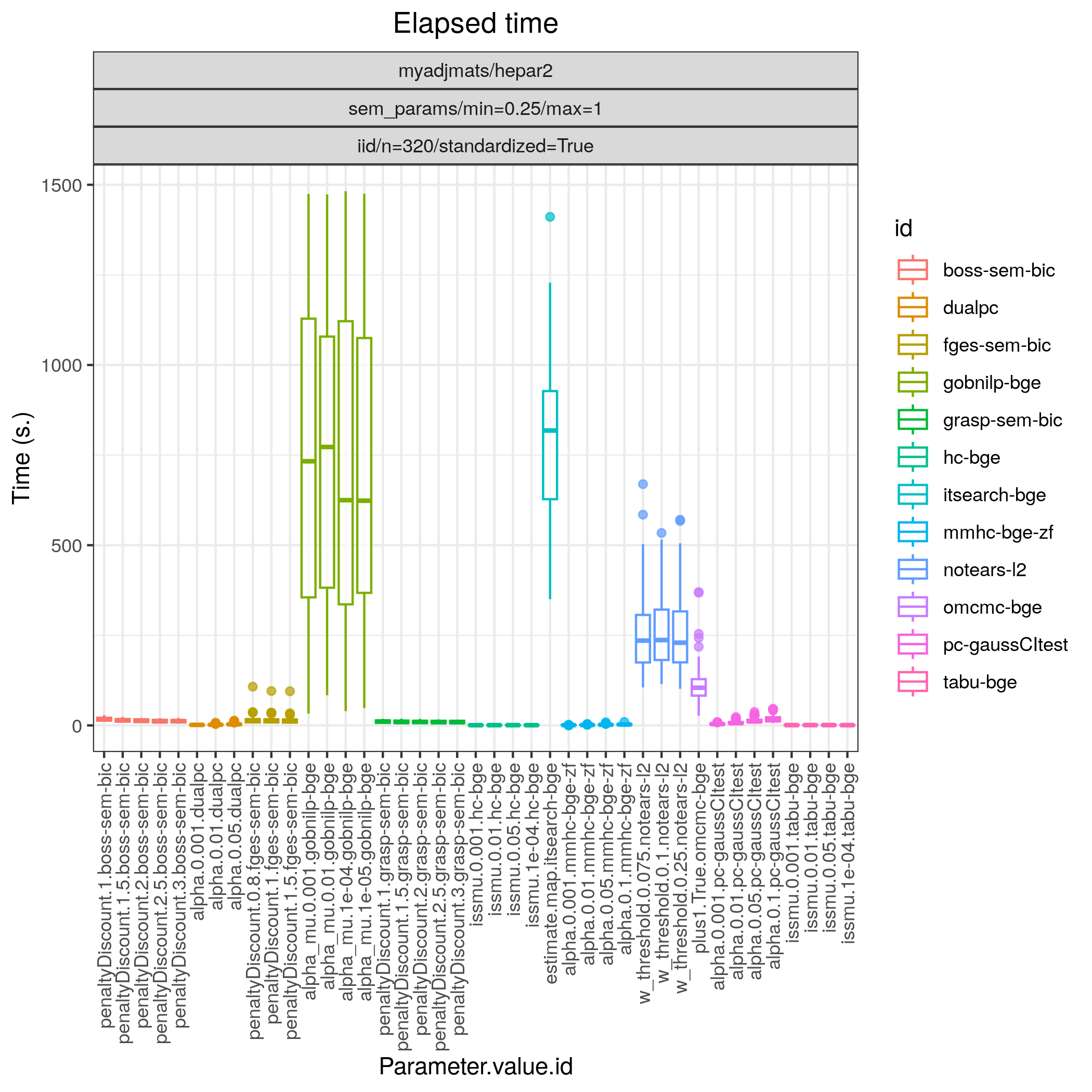
Fig. 13 Timing.
V) Fully generated
The following examples falls into scenario V) Fully generated of the Data scenarios.
Small example
Config file: config/config.json.
Command:
snakemake --cores all --use-singularity --configfile config/config.json
Approximate time: 10 min. on a 3.1 GHz Dual-Core Intel Core i5.
This study is an example of data scenario V) Fully generated based on three continuous datasets, sampled using the iid module, corresponding to three realisations of a random linear Gaussian structural equation model (SEM) with random DAG.
The DAGs are sampled from a restricted Erdős–Rényi model using the pcalg_randdag module and the weight parameters are sampled uniformly using the sem_params module.
For simplicity, we use only a few structure learning modules here, namely Iterative MCMC (BiDAG), FGES (TETRAD), Tabu (bnlearn), and PC (pcalg), with different parameter settings.
The benchmark_setup section of this study is found in Listing 3.
 1"benchmark_setup": [
 2        {
 3        "title": "config",
 4        "data": [
 5            {
 6                "graph_id": "avneigs4_p20",
 7                "parameters_id": "SEM",
 8                "data_id": "standardized",
 9                "seed_range": [1, 3]
10            }
11        ],
12        "evaluation": {
13            "benchmarks": {
14                "filename_prefix": "example/",
15                "show_seed": false,
16                "errorbar": true,
17                "errorbarh": false,
18                "scatter": true,
19                "path": true,
20                "text": false,
21                "ids": [
22                    "fges-sem-bic",
23                    "tabu-bge",
24                    "itsearch-bge",
25                    "pc-gaussCItest"
26                ]
27            },
28            "graph_true_plots": true,
29            "graph_true_stats": true,
30            "ggally_ggpairs": true,
31            "graph_plots": [
32                "fges-sem-bic",
33                "tabu-bge",
34                "itsearch-bge",
35                "pc-gaussCItest"
36            ],
37            "mcmc_traj_plots": [],
38            "mcmc_heatmaps": [],
39            "mcmc_autocorr_plots": []
40        }
41    }
42]
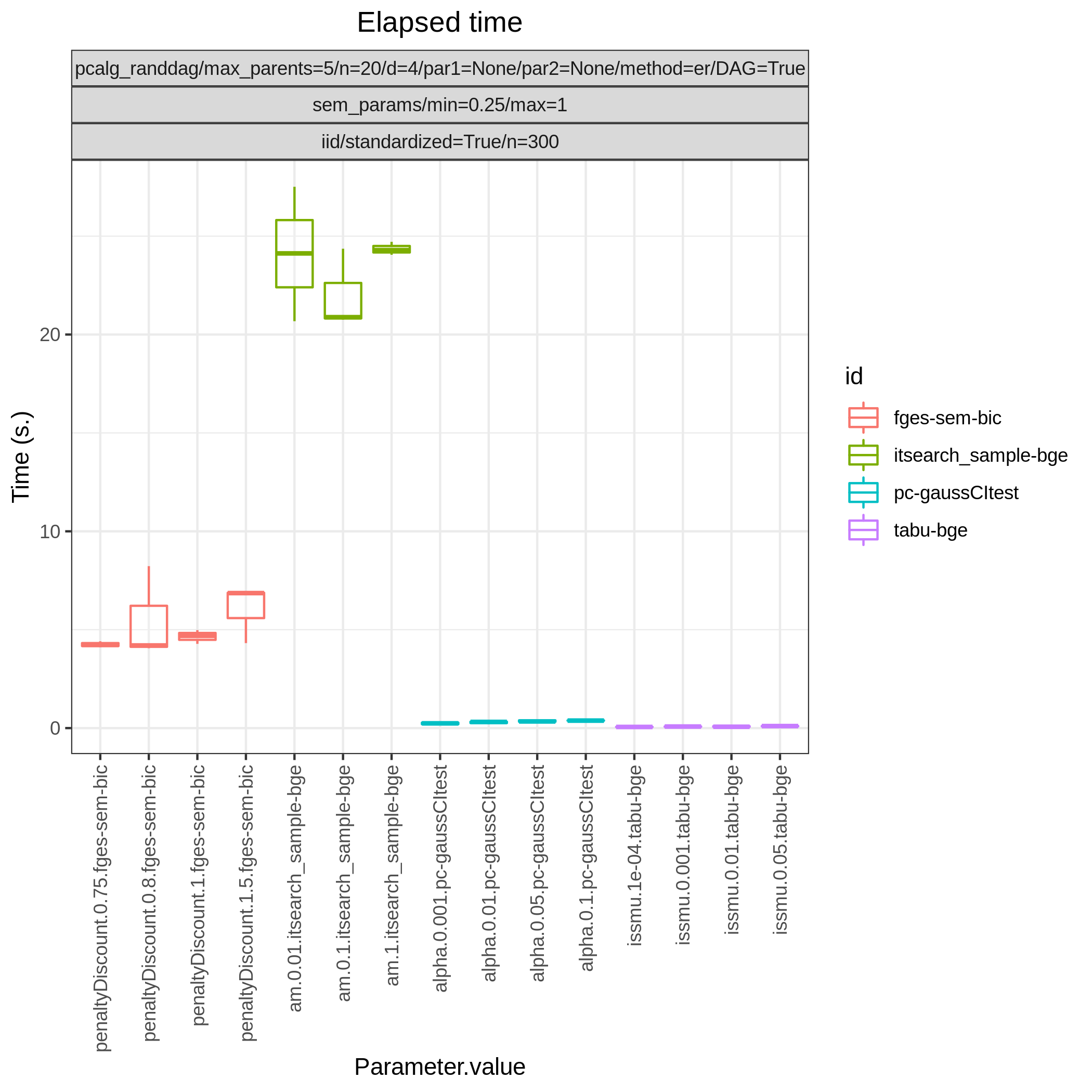
The following plots are generated by the benchmarks module
From graph_true_plots and graph_plots we get
PC vs. dual PC
Config file: config/paper_pc_vs_dualpc.json.
Command:
snakemake --cores all --use-singularity --configfile config/paper_pc_vs_dualpc.json
Approximate time: 20 min.
This is a small scale simulation study from data scenario V) Fully generated where PC (pcalg) and Dual PC (dualPC) are compared side-by-side.
We consider data from 10 random Bayesian network models \(\{(G_i,\Theta_i)\}_{i=1}^{10}\), where each graph \(G_i\) has \(p=80`\) nodes and is sampled using the pcalg_randdag module.
The parameters \(\Theta_i\) are sampled from the random linear Gaussian SEM using the sem_params module with min =0.25, max =1.
We draw one standardised dataset \(\mathbf Y_i\) of size \(n=300\) from each of the models using the iid, module.
The benchmark_setup section of this study is found in Listing 4.
 1"benchmark_setup": [
 2    {
 3    "title": "paper_pc_vs_dualpc",
 4    "data": [
 5        {
 6            "graph_id": "avneigs4_p80",
 7            "parameters_id": "SEM",
 8            "data_id": "standardized",
 9            "seed_range": [1, 10]
10        }
11    ],
12    "evaluation": {
13        "benchmarks": {
14            "filename_prefix": "paper_pc_vs_dualpc/",
15            "show_seed": true,
16            "errorbar": true,
17            "errorbarh": false,
18            "scatter": true,
19            "path": true,
20            "text": false,
21            "ids": [
22                "pc-gaussCItest",
23                "dualpc"
24            ]
25        },
26        "graph_true_plots": true,
27        "graph_true_stats": true,
28        "ggally_ggpairs": false,
29        "graph_plots": [
30            "pc-gaussCItest",
31            "dualpc"
32        ],
33        "mcmc_traj_plots": [],
34        "mcmc_heatmaps": [],
35        "mcmc_autocorr_plots": []
36    }
37}]
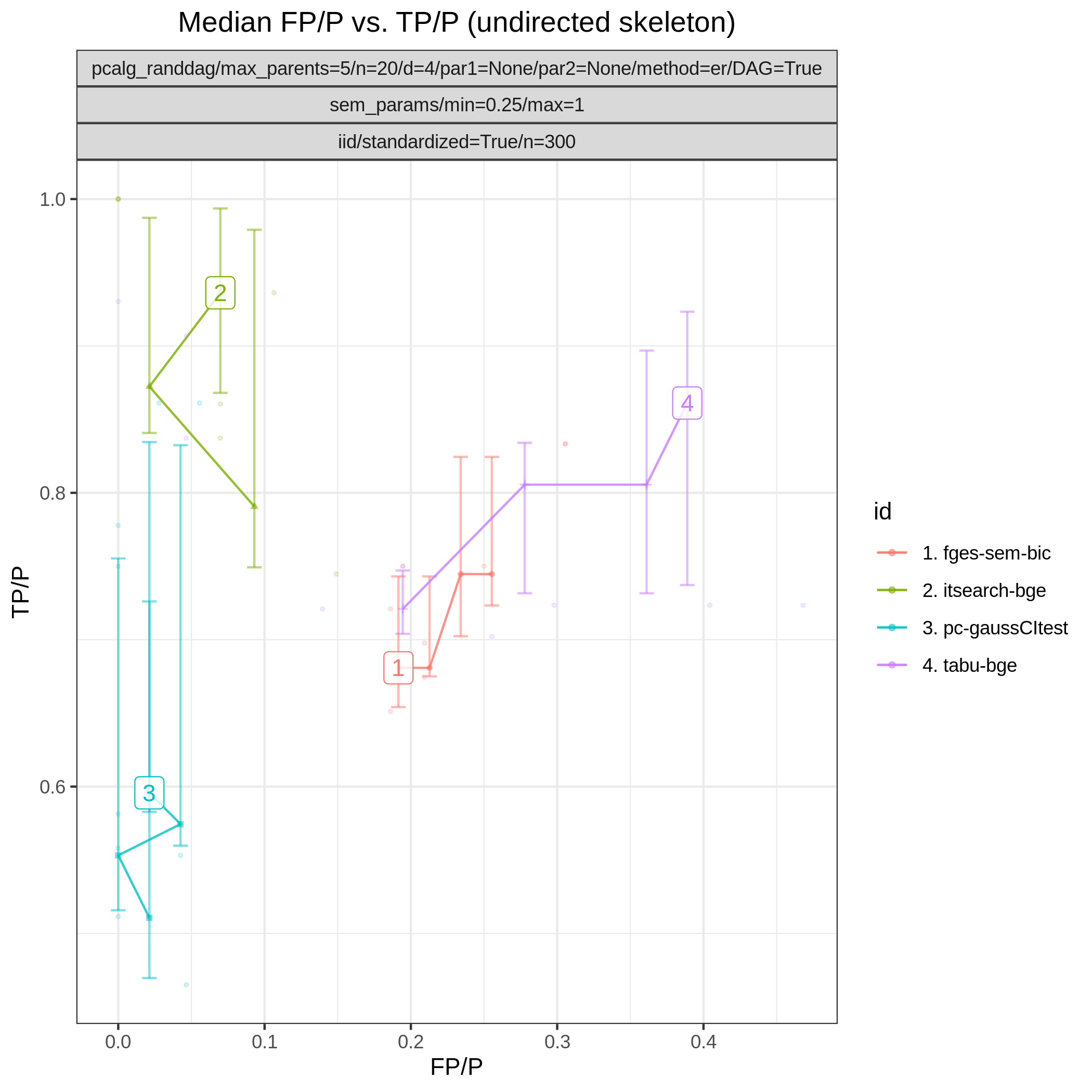
Results from the benchmarks and the graph_true_stats module, where we have focused on the undirected skeleton for evaluations since this is the part where the algorithms mainly differ. More specifically, from Fig. 14, showing the FP/P and TP/P, we see that the dual PC has superior performance for significance levels alpha=0.05,0.01. Apart from the curves, the numbers in the plot indicates the seed number of the underlying dataset and models for each run. We note that model with seed number 3 seems give to good results for both algorithms and looking into Fig. 15, we note that the graph with seed number 3 corresponds to the one with the lowest graph density \(|E| / |V|\). The box plots from Fig. 17 shows the computational times for the two algorithms, where the outliers are labeled by the model seed numbers. We note e.g., that seed number 1 gave a bit longer computational time for the standard PC algorithm and from Fig. 15 we find that the graph with seed number 1 has relatively high graph density. The conclusion of the F1 score plot in Fig. 16. are in line with the FP/P / TP/P results from Fig. 14.
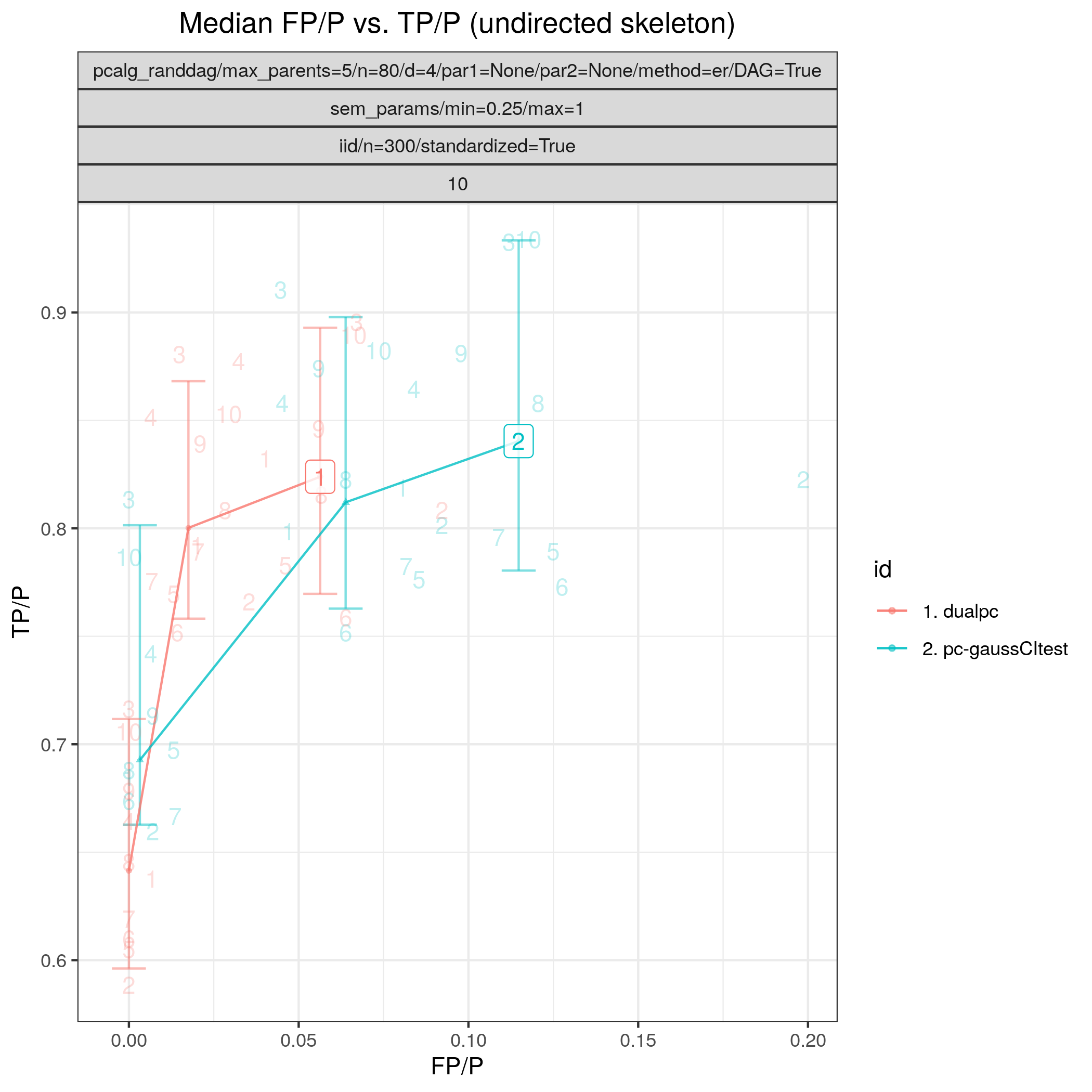
Fig. 14 FP/P vs. TP/P.
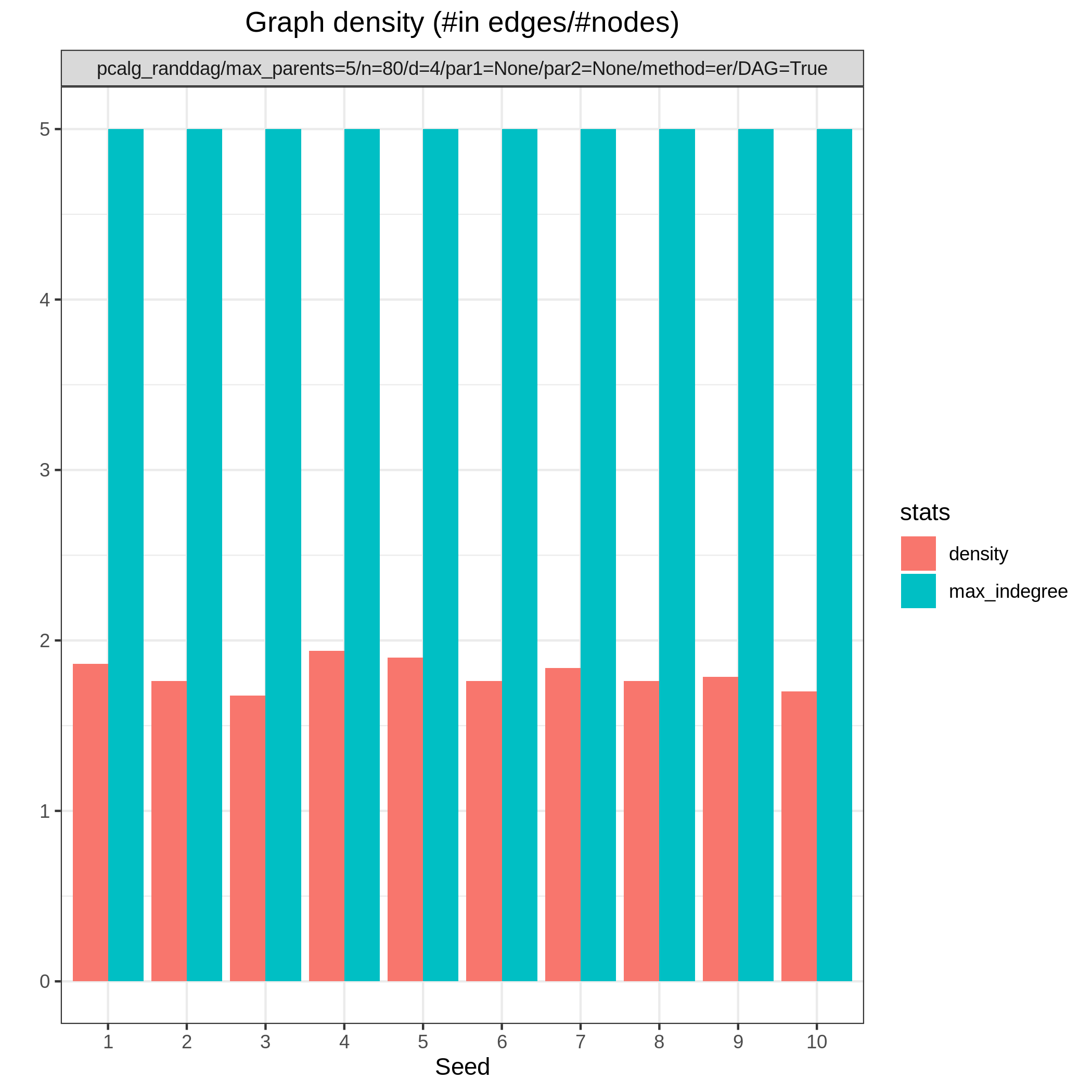
Fig. 15 Graph density.

Fig. 16 F1.
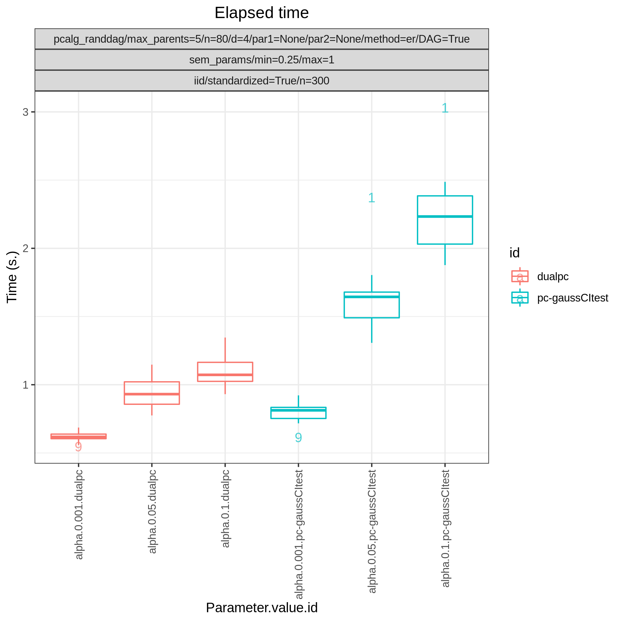
Fig. 17 Timing.
Random Gaussian SEM (small study)
Config file: config/paper_er_sem_small.json.
Command:
snakemake --cores all --use-singularity --configfile config/paper_er_sem_small.json
Approximate time: 40 min. on a 3.1 GHz Dual-Core Intel Core i5.
In the present study we consider a broader simulation over 13 algorithms in a similar Gaussian data setting as in PC vs. dual PC, with the only difference that the number of nodes is reduced to 20 and the number of seeds is increased to 10.
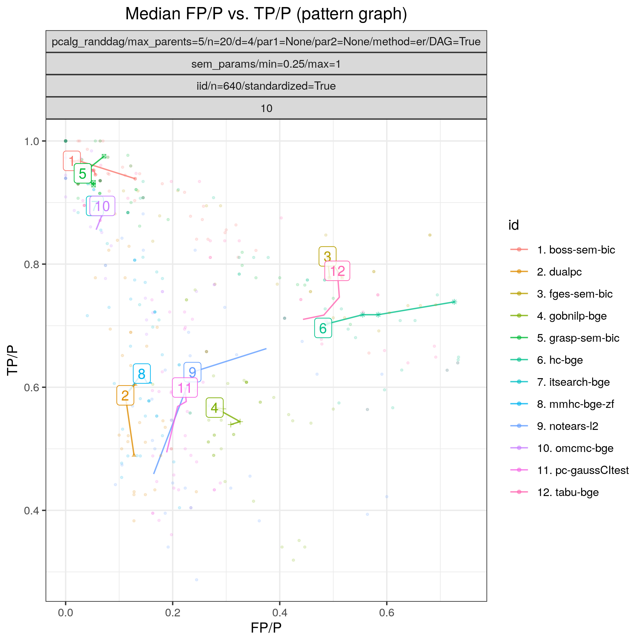
Fig. 18 FP/P vs. TP/P.
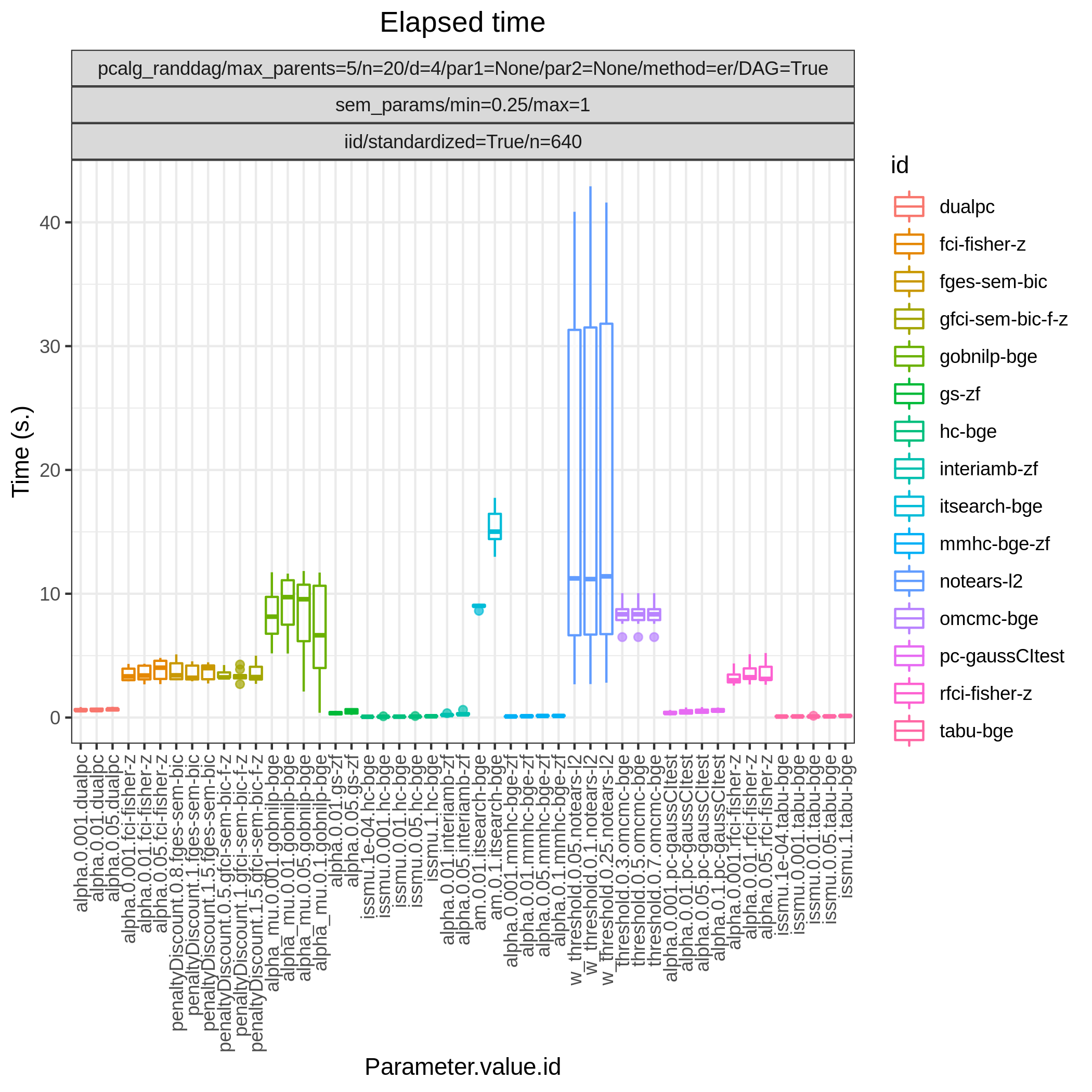
Fig. 19 Timing.
Fig. 18 shows FP/P / TP/P based on pattern graphs and Fig. 19 shows the computational times. BOSS (TETRAD) (boss-sem-bic), GRaSP (TETRAD) (grasp-sem-bic), Iterative MCMC (BiDAG), (itsearch-bge), and Order MCMC (BiDAG) (omcmc-bge) have the best (near perfect) performance.
Random binary Bayesian network
Config file: config/paper_er_bin.json.
Command:
snakemake --cores all --use-singularity --configfile config/paper_er_bin.json
In this example we study a binary valued Bayesian network, where both the graph \(G\) and the parameters \(\Theta\) are regarded as random variables. More specifically, we consider 100 models \(\{(G_i,\Theta_i)\}_{i=1}^{100}\), where each \(G_i\) is sampled according to the Erdős–Rényi random DAG model using the pcalg_randdag module, where the number of nodes is p=80 (p is called n in this module), the average number of neighbours (parents) per node is 4 (2) and the maximal number of parents per node is 5.
"pcalg_randdag": [
    {
        "id": "avneigs4",
        "max_parents": 5,
        "n": 80,
        "d": 4,
        "par1": null,
        "par2": null,
        "method": "er",
        "DAG": true
    }
]
The parameters \(\Theta_i\) are sampled using the bin_bn module and restricting the conditional probabilities within the range [0.1, 0.9].
"bin_bn": [
    {
        "id": "binbn",
        "min": 0.1,
        "max": 0.9
    }
]
From each model, we sample a dataset \(\mathbf Y_i\) of size n=320 and using the iid module.
"iid": [
   {
       "id": "example3",
       "standardized": false,
       "n": 320
   }
]
Fig. 20 shows the ROC type curves for the algorithms considered for the discrete data as described above. The algorithms standing out in terms of low SHD in combination with low best median FP/P (< 0.12) and higher best median TPR (>0.5), are BOSS (TETRAD) (boss-bdeu), GRaSP (TETRAD) (grasp-bdeu), FGES (TETRAD) (fges-bdeu), and Order MCMC (BiDAG) (omcmc-bde).
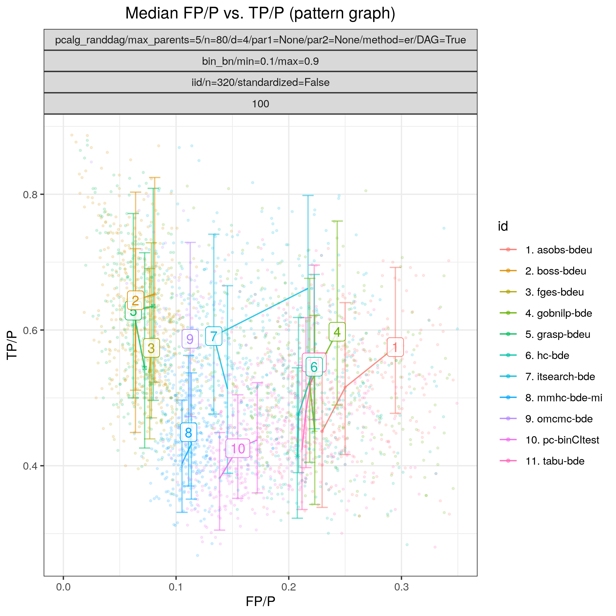
Fig. 20 FP/P vs. TP/P.
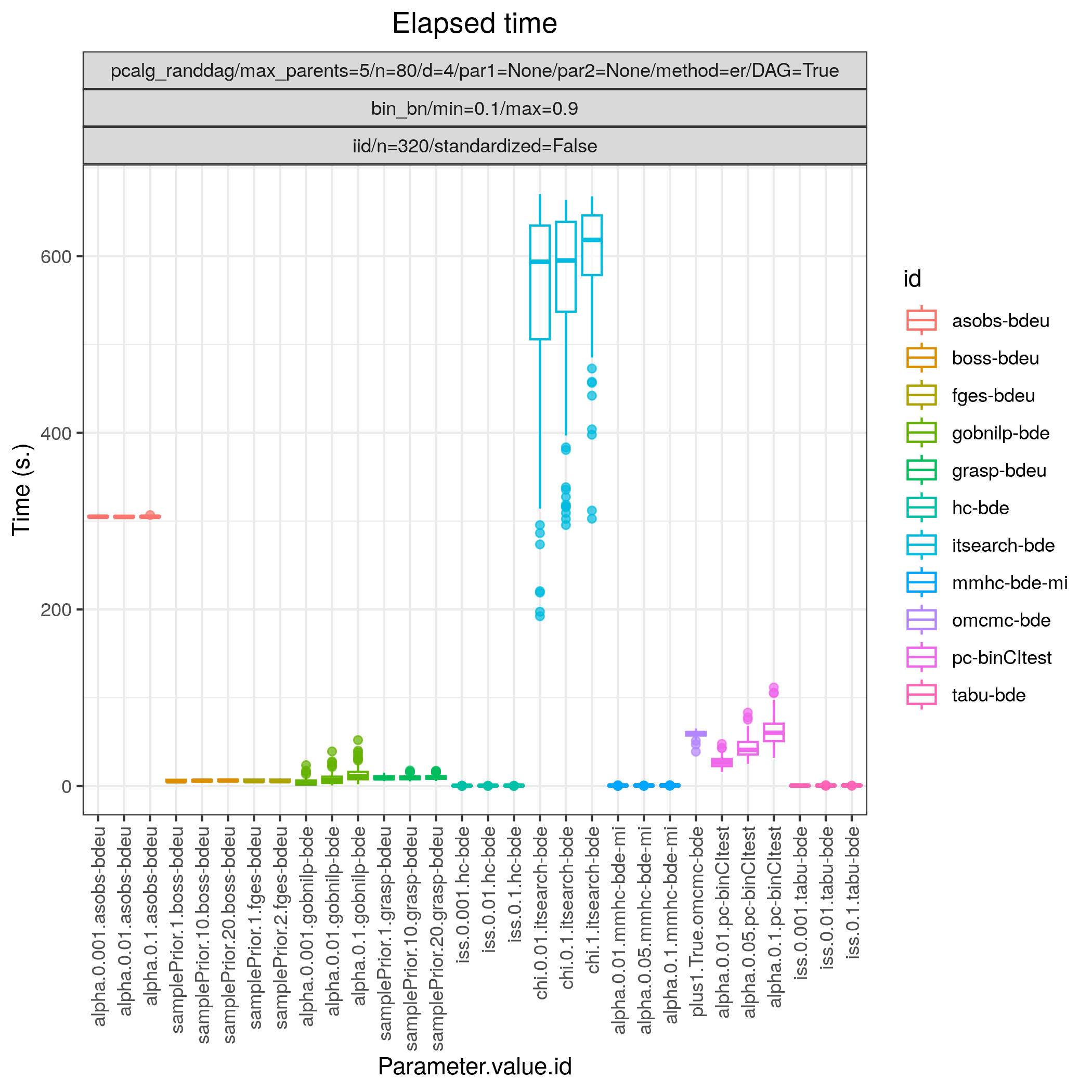
Fig. 21 Timing.
Random Gaussian SEM
Config file: config/paper_er_sem.json.
Command:
snakemake --cores all --use-singularity --configfile config/paper_er_sem.json
In this example we again study a linear Gaussian random Bayesian networks, of size p=80 and with 100 repetitions \(\{(G_i,\Theta_i)\}_{i=1}^{100}\). As in Random Gaussian SEM (small study), we draw a standardised dataset \(\mathbf Y_i\) of size n=320 from each of the models using the iid module.
Fig. 22 shows results for all the algorithms considered for continuous data as described above. In terms of achieving high TP/P (>0.95) Order MCMC (BiDAG) (omcmc_itsample-bge) and Iterative MCMC (BiDAG) (itsearch-bge), BOSS (TETRAD) (boss-sem-bic), and GRaSP (TETRAD) (grasp-sem-bic) stand out with near perfect performance, i.e., SHD \(\approx 0\). Among the other algorithms GOBNILP (GOBNILP) (gobnilp-bge) performs next best for both sample sizes with TP/F \(\approx 0.85\) and FP/P \(\approx 0.05\), followed by FGES (TETRAD) (fges-sem-bic).
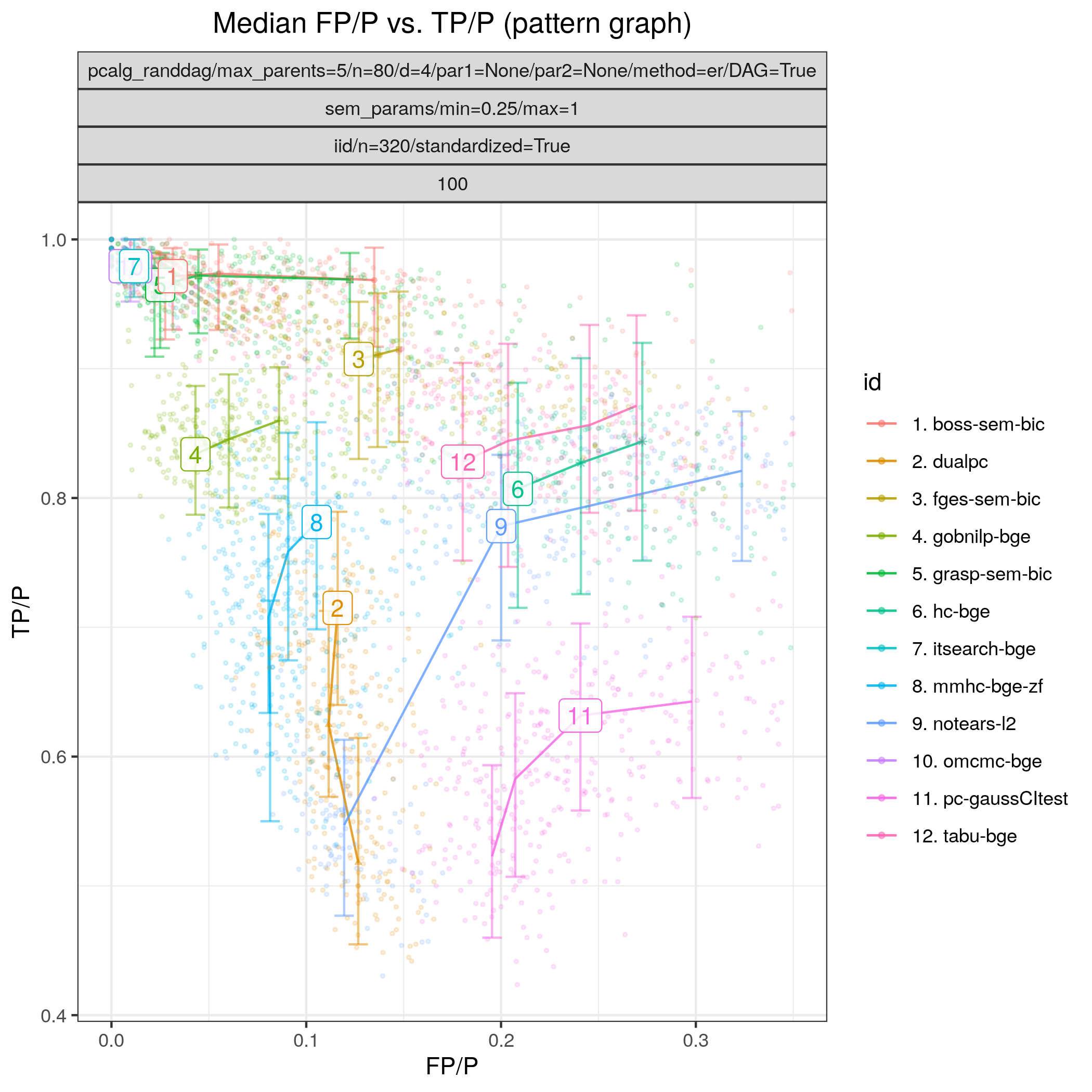
Fig. 22 FP/P vs. TP/P.
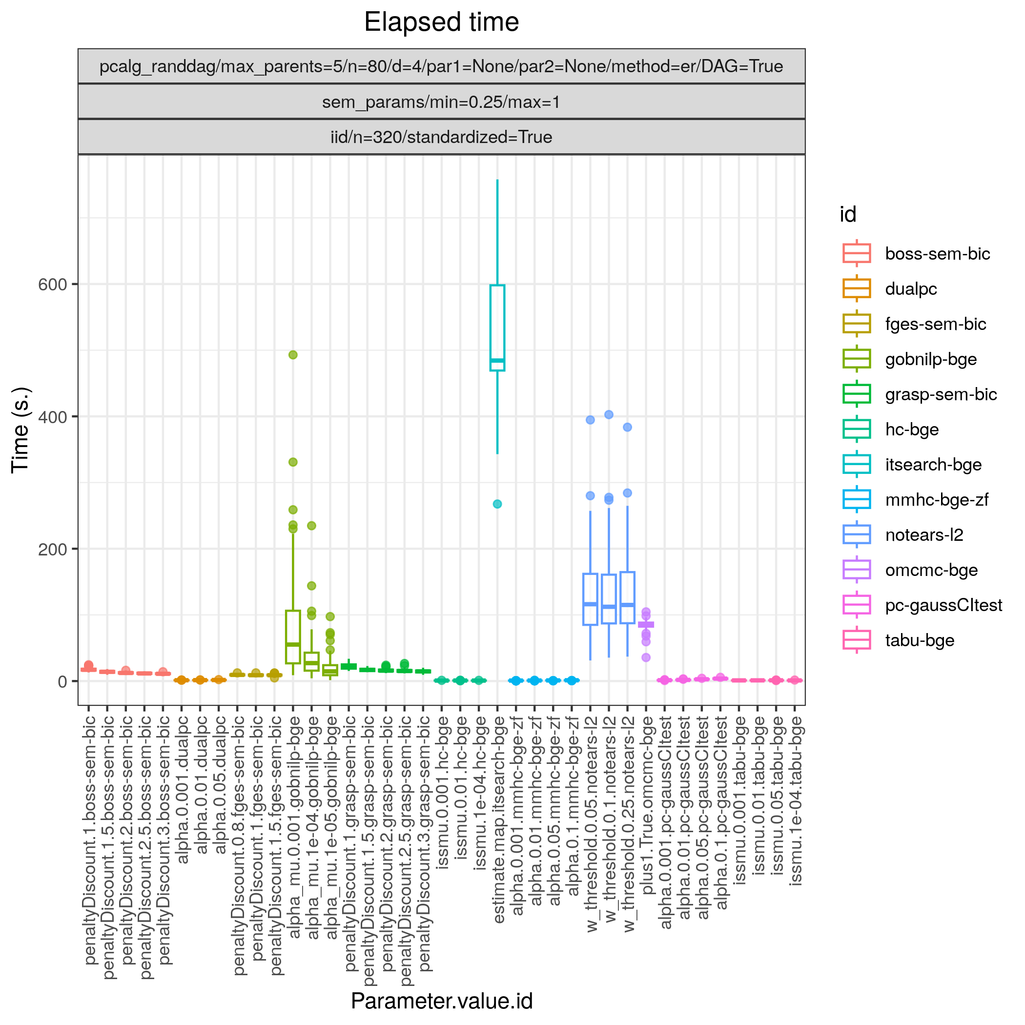
Fig. 23 Timing.